The Peierls argument

There is a great effort in statistical physics in trying to understand phase transitions. A phase transition is characterized by a strong change in the properties of a material, such as a sudden change in magnetization, or specific heat. We are going to see a simple argument which shows some systems must have phase transitions, while others can’t. It is a well known argument due to Rudolph Peierls.

To begin, we have to understand what happens to a system when it is in contact with a reservoir of fixed temperature. Maybe it tries to minimize its internal energy? Or maximize its entropy? What really happens can be seen as a balance between these two principles, in fact it corresponds to minimizing the Helmholtz free energy. This is a thermodynamic potential given in terms of the internal energy $U$ and the entropy $S$ (at a fixed temperature $T$ ) by

$F=U-TS$ .

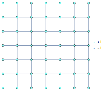
The equilibrium state is that which minimizes the Helmholtz free energy and has the same temperature as the reservoir. Let’s see how this idea applies to a simple and paradigmatic system of statistical mechanics: the Ising model. We have a square lattice, and at each site we place a spin variable, which can have a value of +1 or -1. That is, each spin may point up or down.

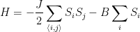
The energy of this system is given by its Hamiltonian. We imagine every spin only interacts with its first neighbors, and the interaction energy is smaller when both spins point in the same direction. A Hamiltonian with these features is

$\displaystyle H = -J \sum_{\langle i,j \rangle} \sigma_i \sigma_j - \sum_i h_i \sigma_i$

$J$ is a positive quantity standing for the interaction energy between spins, and each variable $\sigma_i$ represents a spin at position $i$ . When both are in the same direction, their contribution to the energy is negative, hence it diminishes the total energy. But when neighbor spins are in opposite directions they raise the total energy. Finally, $h_i$ is an external magnetic field at site $i$ .

Now we want to find out the state of minimum free energy, beginning with a 1D system. Let’s start with a lattice with all spins pointing up, this would be an equilibrium state if the system were at zero temperature (all neighbor spins are pointing in the same direction, so the energy is the least possible).

Ising1D_Ordered

If we invert a strip of spins of size $L$ , including a certain spin $X$ , this raises the internal energy of the system by $4 J$ . But this change in energy does not depend on the size of the domain of down spins we created.

Ising1D_Inverted

To account for the entropy difference, we have to count in how many ways this configuration can be arranged. The answer is simple, there are only $L$ ways to make this domain of flipped spins which include spin $X$ . The change in entropy is given by the Boltzmann formula

$\Delta S = k \ln \Omega$ ,

where $\Omega$ is the number of ways the system can be arranged, which in this case is simply $L$ , and $k$ is Boltzmann constant.

Then creating this domain results in a change in free energy of $\Delta F = 4 J - k T \ln L$ , and if the domain is large enough, the second term will always dominate, for it can easily be larger than the first. From this we can see that creating a domain with flipped spins favors the free energy, by lowering it. The system will go to the new state with lower free energy, thus accommodating the created subdomain. Other domains like this are created by thermal fluctuations and eventually disorder the whole system.

Then, in one dimension, disorder always dominates because it lowers the Helmholtz free energy. But in two dimensions the picture is very different. We again start with a completely ordered lattice with spins pointing up

Ising2D_Ordered

and form an island of down spins. This island will be of perimeter $L$ .

Ising2D_Inverted

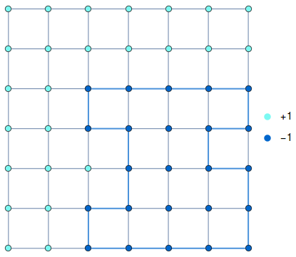
There are misaligned spins all along the border of this region and each spin at the border contributes to a difference of $2J$ in the internal energy. But only these spins contribute to a change in energy. Hence the total energy difference is proportional to the perimeter:

$\Delta U = 2 J L$ .

The numbers of ways to build an island which includes a fixed spin $X$ again is how we compute the change in entropy due to the flipped domain. This number is roughly $\Omega = \mu^L$ , where $\mu$ is a number less than 3, as we are going to see. The change in entropy is then $\ln \Omega$ and finally the change in free energy is

$\Delta F = 2 J L - k T L \ln \mu$ .

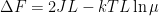
This quantity is linear in L and can be either positive or negative, depending on the temperature the system is in. At low temperatures, $\Delta F$ is positive, and the formation of flipped domains is not favorable, thus the system remains ordered. Whereas at high temperatures, these domains reduce the Helmholtz free energy and disorder wins. The temperature where the change from one behavior to the other happens is called the critical temperature, and is of the order $J/k$ .

This argument illustrates the idea of a lower critical dimension, which is $d_L=1$ for the Ising model and other similar systems (systems with local interactions and with a discrete symmetry). This means no ordered phase may exist at or below this critical dimension, only above it.

A little more about $\mu$

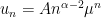
Let’s now investigate the number $\mu$ , which I argued is less than 3. We wanted to draw a closed path of length $L$ on a square lattice. Beginning at position $X$ , there are 4 options of directions to go. We may choose the up direction, for instance.

At the next site, we can’t go back, so there are only 3 options left. For most successive steps, there are only 3 options, or less. Because the path is closed, and we have to be back at the original site after $L$ steps.

At some point, the number of options decreases, forcing us to go back to site $X$ . Hence, the number of paths is bounded by $4 3^{L-1}$ , and we can say it is $\mu^L$ . Mathematically, there is a well defined limit for $\mu$ as the number of steps $L$ approaches infinity, and there are several computational efforts to find this limit with greater precision and enumerate the exact number of possible paths at larger values of $L$ .

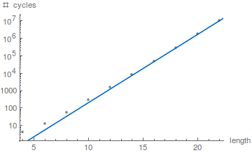
The number of possible paths of length $L$ is an integer sequence available at the OEIS, and we can try to fit the available values to an exponential curve to find the value of $\mu$ . The figure below shows this fit for the few values the list provides, and we can already see a curve very close to an exponential (which is a straight line in a log-linear plot). The value found for $\mu$ is 2.45.

expFit

Recent work on the subject concentrates on enumerating the number of polygons of a certain perimeter and with a fixed site. This is a little different from the problem we are studying, which is the number of cycles of a certain perimeter, rather than polygons. The difference is that polygons are not oriented, neither have a special vertex which is the starting point. In the figure below, we see all polygons of perimeter 8, for instance.

IsoperimetricPolygons

But these two problems are closely related: If $u_n$ is the number of cycles of lenght $n$ and $p_n$ is the number of polygons of same length, they are connected by

$u_n = 2 n p_n$ .

This formula can be easily proved: In the polygon of length $n$ , any of its sites can be the starting site for a cycle, hence the factor $n$ , and for every starting position there are two directions to follow, clockwise or counter clockwise, and we get the factor 2. The number we are seeking is the number of cycles $u_n$ .

Nowadays we know the number of cycles grows as approximately

$u_n = A n^{\alpha-2} \mu^n$

and the best values for these quantities are $\alpha = .5$ and $\mu=2.638$ . So we see $\mu$ is indeed less than 3, as observed. This is a much more precise value than the naive estimation of 2.45 we did.

Some references

Herbert B. Callen, “Thermodynamics and an Introduction to Thermostatistics” (1998)
If you want more details on why we minimize the Helmholtz free energy $F$ .
John Cardy, “Scaling and renormalization in statistical physics, Vol. 5” Cambridge university press (1996)
If you want to go beyond the Peierls argument.
Iwan Jensen and Anthony J. Guttmann, “Self-avoiding polygons on the square lattice”, Journal of Physics A: Mathematical and General 32.26 (1999)
To know more about the numerical study on the value of $\mu$ .
The OEIS
Has sequences for both the number of cycles and of polygons on the square lattice.

Source code

The source code is provided on Github under the MIT license.

The epsilon expansion and the Ising model

The Ising model is the paradigmatic example in the theory of phase transitions and critical phenomena, because it is the simplest statistical model with phase transitions. Its simplicity is in replacing spins on a lattice by scalars with the value $\pm 1$ .

It is close enough to a real description of a spin system and simple enough to be solved exactly in some cases, and the Hamiltonian is:

$\displaystyle H = - \frac{J}{2} \sum_{\langle i,j \rangle} S_i S_j - B \sum_i S_i$

Close to the critical point, the response functions of a statistical system behave as power laws, the correlation length as an example:

$\xi \propto |t|^{-\nu} \ \mbox{at} \ B = 0$

$t$ is the reduced temperature $T-T_C / T_C$ . And $T_C$ is the critical temperature, where a phase transition happens.

We are going to see how the epsilon expansion is used to find the above critical exponents in the Ising model close to four dimensions. Up to first order, it’s easy to do this, using just some power counting and without the need of path integrals.

In four dimensions, it is better to treat the spins as continuous variables, but still with a distribution peaked around $\pm 1$ . The Hamiltonian corresponding to this is:

$H = \int \mathrm{d}^d r \frac{1}{2} (\nabla S)^2 + t S^2 + u S^4 + h S$

It seems a really drastic modification, but it’s justified since we are only interested in calculating universal quantities. Critical exponents, that is. As long as we don’t leave the Ising universality class, these universal observables don’t change. The renormalization group takes us from one theory to another in the same universality class, but often making calculations much easier. Universal quantities obtained are exactly equal to the ones in the original model, not approximately.

The $\epsilon$ expansion relies on the existence of two fixed points that are close and related by a small parameter ( $\epsilon$ ) with which we can make expansions. This parameter is usually related to the dimensionality of the problem and in our case it is $\epsilon = 4 - d$ .

In $d=4$ , $t$ and $h$ are the relevant scaling variables, called thermal and magnetic. The symmetric (coupled to $S^2$ ) is the thermal one, and $h$ is the magnetic one, coupled to the odd operator $S$ . Comparing with the discrete Hamiltonian we can intuitively justify these names.

The scaling variable $u$ is marginal in 4 dimensions, that is, its scaling exponent is $y_u = 0$ . This means the system is in its upper critical dimension. In dimensions above this one, simple mean field theory can be applied.

To show the upper critical dimension is $d=4$ , we are going to find the dimensions of each operator in the Hamiltonian. The action is dimensionless, a way to see this is by noticing that the partition function is given by

$\displaystyle Z = \mathrm{Tr} {}_S \ e^{-H}$

and since $H$ is the argument of an exponential, it must be dimensionless. This permits us to find the engineering dimensions of the fields. From the kinetic term in the action, the derivative accounts to $a^{-2}$ and the integral to $a^d$ :

$[\phi]^{2} a^{d-2} = 1 \mbox{.}$

Hence

$[\phi] = a^{1-d/2} \mbox{.}$

This is used to deduce the dimensions of the scaling variables: $[t]=a^{-2}$ , $[h]=a^{-1-d/2}$ and $[u]=a^{d-4}$ . If we change the spacing as $a \rightarrow b a$ , to this order, the parameters must be changed in the following way to keep the action invariant:

$t' = b^2 t \mbox{,}$

$h' = b^{d/2+1} h \mbox{,}$

$u' = b^{4-d} u \mbox{.}$

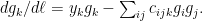
This justifies the renormalization group equations to order zero. In our case, we are making an infinitesimal dilation $b = (1 + \delta \ell)$ , where $\delta \ell$ is a small parameter. With a Taylor expansion, we obtain the first piece of the renormalization group equations:

$dh/d \ell = (d/2 + 1) h \mbox{,}$

$dt/d \ell = 2 t \mbox{,}$

$du/d \ell = \epsilon u \mbox{.}$

Where $\epsilon = 4 - d$ .

To go on to second order we are going to need something called the operator product expansion. Consider the correlation function

$\langle \phi_i (r_1) \phi_j (r_2) \Phi \rangle$ ,

where $\Phi$ is a product of operators $\Pi_l \phi_l (r_l)$ , and we would like to know the behavior of this correlation function in the limit when $|r_1 - r_2|$ is much smaller than $|r_1 - r_l|$ , $l$ pertaining to the product in the operator $\Phi$ .

The idea of the OPE is that this can be replaced by

$\displaystyle \sum_k C_{ijk}(r_1 - r_2) \langle \phi_k(r_1) \Phi \rangle \mbox{,}$

This is the operator product expansion (OPE). And it has been verified in many exactly solvable models. This identity can be written in a loose sense as:

$\displaystyle \phi_i \phi_j = \sum_{ij} C_{ijk} \phi_k \mbox{,}$

keeping in mind that this is only valid when this expression is inserted in a correlation function satisfying the above hypotheses.

Symmetry and scaling arguments leads one to show

$C_{ijk} = \frac{c_{ijk}}{|r_1 - r_2|^{3 d - y_i - y_j + y_k}} \mbox{.}$

And the perturbative renormalization group tells us that the RG equations for
the epsilon expansion up to first order are:

$d g_k / d \ell = y_k g_k - \sum_{ij} c_{ijk} g_i g_j \mbox{.}$

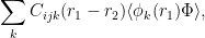
We already have the $y_k$ and the coefficients in the OPE can be found simply by combinatorics as we are going to see.

To find the OPE of $\phi_n$ and $\phi_m$ , draw them as sets of $n$ and $m$ points, respectively. Using Wick’s theorem, each operator can be contracted with another one or with the operator $\Phi$ , drawn as a big distant circle.

In $\phi_2 \phi_2$ , for example, there are three possibilities, shown in the diagram.

diagrams_OPE_Ising_2

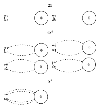
All dots can be linked from $\phi_2$ to $\phi_2$ in 2 ways. To the external operator, this looks like just a number multiplied by the identity operator $1$ .

There can be one link only and there are 4 ways of doing this. The other two dots look like a single $\phi^2$ operator, for they are close together and distant enough from $\Phi$ .

Finally, the last option is no internal links, making the 4 dots look like a $\phi^4$ operator to $\Phi$ . There is only one way of doing this.

Hence, the operator product expansion is:

$\phi_2 \cdot \phi_2 = 2 + 4 \phi_2 + \phi_4$

All operators $S^m$ above $m=4$ that are generated might be ignored, for their dimensions are $a^{-m}$ and they are irrelevant.

This is what is needed to write the renormalization group equations up to first order. With them, we have the phase diagram of the Ising model, exhibiting two critical points:

$dh/d \ell = (d/2+1) h - 2 \cdot 2 h t + \cdots$

$dt/d \ell = 2 t - h^2 - 4 t^2 - 2 \cdot 12 t u - 96 u^2$

$du/d \ell = \epsilon u -t^2 - 2 \cdot 8 t u - 72 u^2$

The first fixed point is simply $t=0$ , $h=0$ and $u=0$ , this is called the Gaussian fixed point, for the Hamiltonian reduces to a simple free field when all couplings are null. The other fixed point is found to be $h^*=0$ , $u^*=\epsilon/72+\mathcal{O}(\epsilon^2)$ and $t^*=\mathcal{O}(\epsilon^2)$ . Notice that contributions with $i \neq j$ are counted twice.

The thermal eigenvalue is also modified to order $\epsilon$ . The RG equation for $t$ can be written as:

$dt/d \ell = 2 t - 2 \cdot 12 t u^*$ .

And to fist order the coefficient of $t$ is now $y_t = 2 - (24/72) \epsilon + \mathcal{O}(\epsilon^2).$

With these eigenvalues, one can find all the critical exponents. The one we are calculating is:

$\nu = \frac{1}{y_t} \mbox{.}$

Finally, the result desired is in 3 dimensions. It may seem absurd to set a small parameter equal to one, and even more absurd that the approach works to higher orders. It is unfair to compare the values we obtained to the best ones there are, some of those obtained with the renormalization group up to the 5th order,but the result is rather good for the $\nu$ exponent.

Mean field theory predicts $\nu=.5$ , our first order RG predicted $.6$ and the best value is close to $.63$ , hence the result was surprisingly good in this case.

To check out more on the subject, take a look at these books.

John Cardy, Scaling and Renormalization in Statistical Physics
A unique and witty book, brings real insight.

Giuseppe Mussardo, Statistical Field Theory: An Introduction to Exactly Solved Models in Statistical Physics
A more rigorous book, very well written as well and has great epigraphs.